Introduction

We live in a world that is continuous: our eyes see scenes defined by continuous curves and intensities of colors, hear sounds formed by continuously varying pressure waves, and we sense velocity and temperature as continuous signals. In contrast, our computers operate in a discrete world, despite the continuous nature of the world at the scale our senses perceive. We finely divide time and space into quanta in order to model the real world on our digital computers. The inherent costs of digital computing have been ameliorated by digital computers’ exponential growth in computing power relative to energy consumption and size. However, as scaling in digital computers comes to an end, we must explore alternatives to digital, discrete computing.

Our work explores using analog electronic circuits to assist conventional digital computers to obtain high performance and low energy computation. Our prototype analog co-processor solves nonlinear and linear systems of equations, delivering approximate solutions which are useful in physical simulations and machine learning tasks. Commonly perceived downsides of analog computing, such as low precision and accuracy, limited problem sizes, and difficulty in programming are all compensated for using methods we discuss. Based on our findings, small-scale uses of analog computing can bring efficient physics simulation to energy-efficient, Internet-of-Things devices. On the other hand, large-scale uses of analog computing can speed up the training of machine learning applications.

How a nonlinear PDE becomes nonlinear algebra

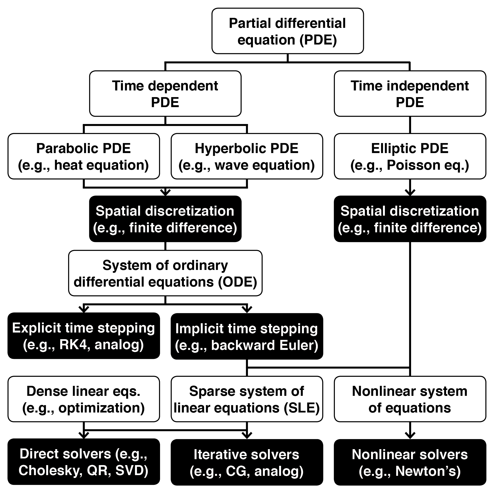
Nonlinear partial differential equations appear in physics simulations. The PDEs are first discretized in space and time. The problem becomes finding an unknown vector x satisfying the system of equations:

F(x) = 0

Nonlinear PDEs are often simplified with linear approximations. For example, linear springs replace realistic springs in solid mechanics; linear dynamics and quadratic costs replace generic models in control theory. With these simplifications the problems become:

Ax–b = 0

Which are efficiently solved using linear algebra algorithms. We seek to provide a nonlinear algebra solver using analog-digital co-processing.

How to solve an ODE using analog circuitry

Analog computers solve ordinary differential equations. Their most important components are integrators that store and output time-dependent variables, and take their derivative as input. Variables are multiplied, summed, and subjected to nonlinear functions (implemented here as digital lookup tables). The integrators are charged to an initial value. Upon release, the variable x is solved according to the ODE. Our team has solved ODEs for embedded systems using an integrated circuit analog co-processor.

Solving linear systems of equations in analog

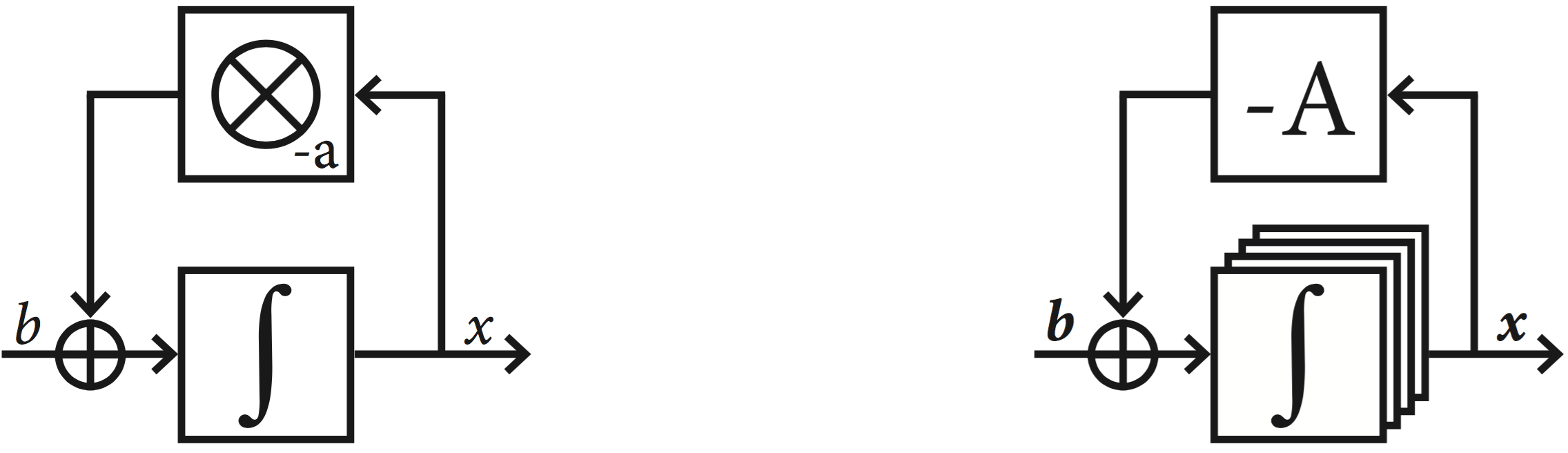
We can solve other problems by converting them to ODEs solved on an analog computer. For example, analog computers can use negative feedback to compute quotients: ax–b = 0. As long as a is positive, the circuit here has x tending toward the stable solution
x = b/a, at which point the summing point at the input of the integrator becomes zero.

This technique can solve linear algebra problems,
Ax–b = 0. Using a vector of integrators and a matrix of multipliers, the circuit here has the integrators’ output tend toward x = A^-1b, as long as A is positive definite.

Our team has solved sparse linear algebra problems appearing in linear PDEs using an integrated circuit analog co-processor.

Applications

Software, programming & architecture

Hybrid Continuous-Discrete Computer Architectures